The Maths Behind Bitcoin: Let's get geometrical

This article is part of a series exploring the maths behind Bitcoin and it will not mention any cryptography, any cryptocurrency or anything cryptic at all (okay, maybe just a bit of maths — but that’s what you’re here for, aren’t you?). If you missed the introductory article, please go check it out.

Photo by Alex Holyoake on Unsplash

The goal here is for you to understand enough geometry to feel comfortable reading the next articles about elliptic curves. You will learn about coordinate systems or how to record a Chess game; you will discover the commitment that any two points make to each other (not so exclusive, huh?), namely lines. You will touch on a bit of set theory to realise what a curve is. We will go on a tangent, and end this article with a bit of fun with squares.

Recording a Chess game

Chess is this game that relies on moving pieces on a 8x8 board and the goal is to capture the opponent’s king to win the game. There are pawns, kings, queens, bishops, knights and towers. Sounds more exciting than Battle Royale, don’t you think? Computers also know how to play and they can even beat the best human chess players!

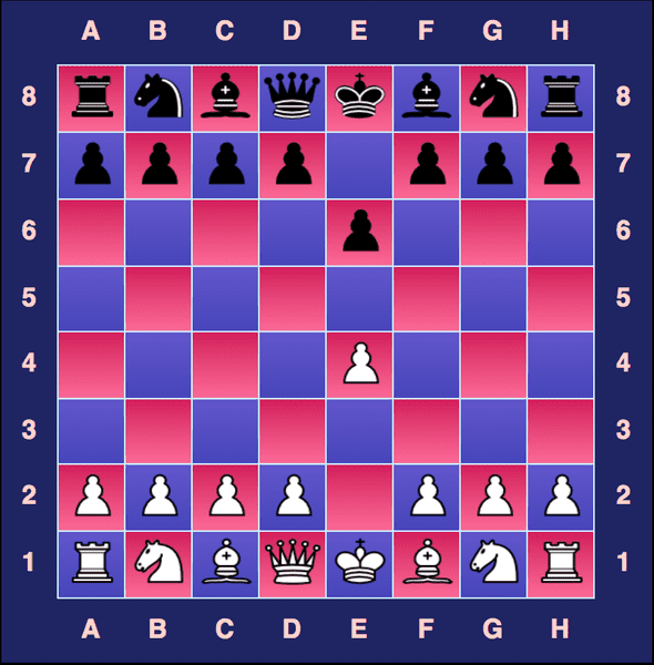
This what a board looks like at the start of the game:

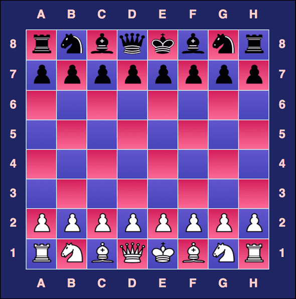Initial chess board configuration

The opening move could be any of the light pawns going one square or two squares towards the dark pawns. Let’s say the first player moves the pawn in front of their king two squares towards the dark pawns. The second player replies with a well-known opening called French defense, by also moving the pawn in front of their king one square towards the light pawns.

French defense opening

Imagine now you are in charge of recording a chess game for posterity (there could be some really interesting strategies or tactics): do you think there could be a better way of describing the moves? We could record every piece’s move with →, ←, ↑ and ↓. For example

light pawn in front of king ↑↑
dark pawn in front of king ↓
...
light knight ↑↑→
...

However, some questions quickly arise:

• is a knight going ↑↑→ or →↑↑?
• is a bishop going ↑→↑→ or →↑→↑?

If we have different ways of representing the same thing, it might quickly become hard to read if we do not follow one convention.

Enter coordinate systems

We can do better than that and write the previous moves as:

E2-E4
E7-E6

meaning the piece at location $E2$ moves to $E4$, and the other piece at $E7$ moves to $E6$.

If we agree on some common context to reason about these moves, this system is enough to describe all chess moves. We will agree that the vertical axis of the board is labeled by letters A, B, C, D, E, F, G, H and the horizontal axis of the board is label with numbers 1, 2, 3, 4, 5, 6, 7, 8. Each square of the board now has a name, eg. $E3$, and we can forget about up-up-right or right-up-up to mean the same move as $E3$ to $C4$.

As an aside, we also need to consider that the moves are recorded in an orderly fashion; otherwise, how do we know this move is allowed if we cannot verify what piece we are talking about? If you’re interested, you can check out the numerous ways to record chess moves.

Well, the same is true for geometry. If we want to reason about points, lines, curves, circles, triangles, we need to agree on some context or way to represent this information somewhat accurately and without ambiguity. In the context (get it?) of this article, we will use the Cartesian coordinate system.

Cartesian coordinate system

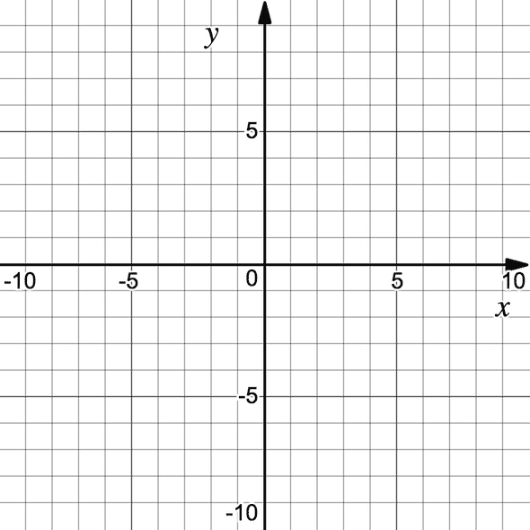
The horizontal axis is commonly called the $x$-axis and the vertical axis the $y$-axis. The points will be labelled under the form $(x, y)$, just like before we had E3 to mean $(E, 3)$; $x$ is the horizontal coordinate and $y$ is the vertical coordinate. In our case, $x$ and $y$ can be any number, like $1, -3, 5,$ but also like $2/3$, $\sqrt{17}$, $\pi$, $e$. Of course, there are other ways to represent a point:

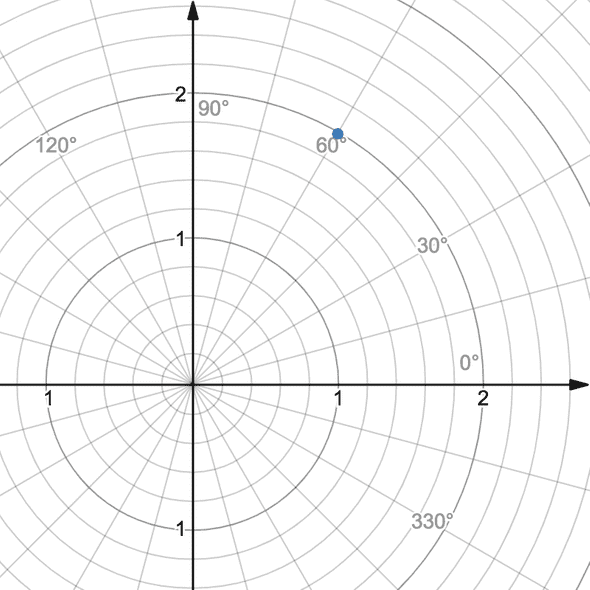The blue point has polar coordinates $(r, \theta) = (2,60°)$ and Cartesian coordinates $(x,y) = (1,\sqrt{3} )$

We will however stick to $(x, y)$ coordinates to talk about points on the plane.

Any two points commit through a line

We’ve all learnt at school that for any 2 points on the plane, there exists a line passing through them. But let me ask you: what is a line exactly? Pause for a moment and try to define what it is in your own words.

This is not a line, René Magritte

When you really look at it and zoom in, you might just see that you just drew a collection of points and they are all so close to each other that what you see is a line.

This is actually how you would write it with mathematical symbols:

Let’s go through these notations:

• $(AB)$: the line passing through points A and B;
• $\{ \text{ things } | \text{ properties} \}$: the set of things with these properties;
• $\mathbb{R} \times \mathbb{R}$: all the pairs of (real) numbers;

So mathematical expression $(1)$ above means: the line passing through points $A$ and $B$ is the set of points $(x,y)$ such that $(x,y)$ is point $A$ or $(x,y)$ is point $B$, or dot-dot-dot. We need to determine this dot-dot-dot to get the full picture.

Algebra to the rescue

Don’t leave just yet, we are getting started! Algebra is where the juice is, you do not want to miss it. Saying that there is a line joining any two points means that any two points have a relationship, namely that $(x_A, y_A)$ is related to $(x_B, y_B)$ in some way. Algebra will help us understand that relationship more precisely.

Algebraically, a line is indeed an equation:

which expresses the value of $y$ depending on the value of $x$, given parameters $a$ and $b$. Parameter $a$ is called the slope and parameter $b$ is called $y$ at the origin.

Let’s have a look at a few examples to understand better what $a$ and $b$ mean.

Graph $y=3$

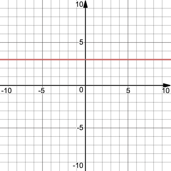
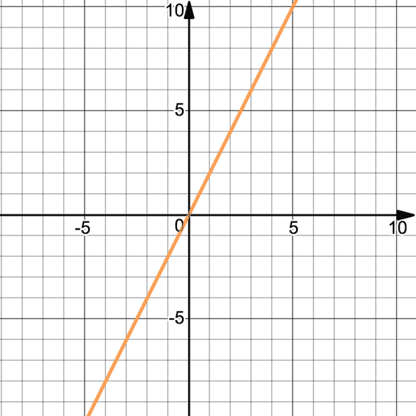
On the line $y = 3$, since it is not depending on $x$ we have $a = 0$, and so $b$ must be $3$. We obtain that not depending on $x$ means $y$ has a constant value and this translates into a horizontal line geometrically.

Graph $y=x+3$

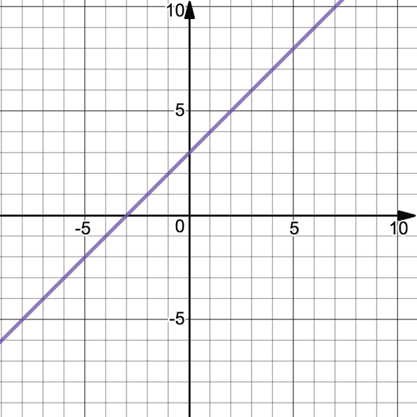
On the line $y=x+3$, we have $a=1$ and $b=3$. We can see that the point with coordinates $(0,3)$ is also being passed through.

Specifying $b$ is the same as saying that the line must pass through the point with coordinates $(0,b)$.

(That’s incidentally why $b$ is called y at the origin.)

Graph $y=2x$

Finally, on the line $y=2x$, we can see the line passes through $(0,0)$, which means $b=0$, and we also have $a=2$. Note that the slope of the line is steeper than the line $y=x+3$.

Joining algebra and geometry, we can write that a line is a set of points $(x,y)$ satisfying the equation $y=ax + b$. Going back to the idea that there is a line passing through any two points, we can rephrase it by saying: there are numbers $a$ and $b$ such that $y_A = ax_A + b$ and $y_B = ax_B+b$, for any two points $A(x_A, y_A)$ and $B(x_B,y_B)$. The following equations must be true simultaneously

which we could rewrite

which means in particular

so that finally

Now that we know $a$, we can find $b$:

To summarise, we found:

Let us use these formulae to obtain the equation for the line passing through points $A(0,3)$ and $B(5,8)$:

and thus $a= \frac{5}{5} = 1$ and $b= \frac{15}{5} = 3$.

The line passing through $A(0,3)$ and $B(5,8)$ has equation

Looks familiar?

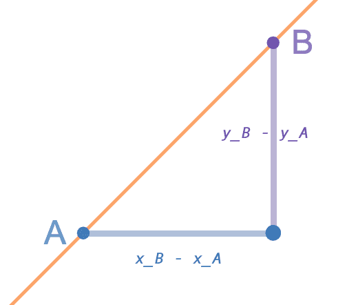
Before moving on to curvy lines, let us understand why $a$ is called the slope.

From the equation we obtained for number $a$, we can visually identify the quantities $x_B-x_A$ and $y_B - y_A$:

• $x_B-x_A$ corresponds to the distance along the $x$-axis to go from $A$ to $B$, and
• $y_B-y_A$ corresponds to the distance along the $y$-axis to go from $A$ to $B$;

In some sense, $a$ measures how much $y$ grows/shrinks as $x$ grows, and it could be expressed in percents like on road signs.

A slope $a = -0.1$, Photo by WikimediaImages on Pixabay

Curvy lines

Rewriting once again our representation of a line as

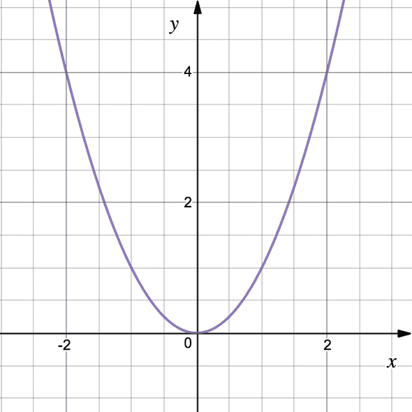
with $f(x) = a x + b$, we see that we are using a very specific function of $x$. We could change it to

and obtain the set $\{ (x,y) \in \mathbb{R}^2 | y = x^2 \}$. This set corresponds to the parabola:

The parabola, aka $y=x^2$

To generalise further, we could write $y = x^2$ as $y - x^2 = 0$. That means we can consider functions of $x$ and $y$ to describe other sets of points:

It is for example useful to describe a circle. A circle is defined as the set of all the points lying at the same distance $r$, called the radius, of another point $C$, called the centre of the circle.

Taking the centre to be $C(0,0)$ and the radius $r$ to be 1, $f(x,y)$ can then be expressed as

This form of expressing sets of points will be useful when talking about elliptic curves in the next article.

(Spoiler alert: $f(x,y)= y^2-x^3-7$ for Bitcoin!)

Let’s go on a tangent

Now that we understand lines and curves a bit better, let’s discuss this special kind of lines called tangents at a point to a curve. These lines will be necessary for us to define a group structure on elliptic curves, which will be the subject of the next article.

Let’s go over the intuition behind them first.

Let’s say you went for a run and your smart watch collected your GPS position. You would like to know your average speed and also your instantaneous speed at some specific point in time.

To compute your speed, you would typically divide the total distance by the time it took.

Computing your instantaneous speed is somewhat similar: you divide the total distance done at that point in time by the time it took.

Oh wait.

How long is an instant? Pretty much zero seconds.

How can we divide by zero then?

To go around this problem, let us relax our requirements a little. What if you instead take two points really close to that point in time and you divide the distance by the time?

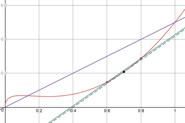
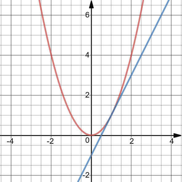
Imagine that the red curve below describes the distance you covered versus time. (Okay, it’s not strictly increasing but let’s assume it is.) We are interested in your instantaneous speed at $t=0.7s$.

As mentioned in the previous paragraph, we could take the points at $t_0 = 0.6s$ and $t_1 = 0.8s$, compute parameter $a$ of the line passing through the corresponding points on the red curve:

and we would obtain an idea of the velocity around this time.

However, we would like to know the velocity at that precise moment when $t=0.7s.$

So let’s move the two points along the red curve closer and closer to the point on the curve where $t=0.7s$. Compute the slope of the resulting line passing through these two points and you obtain an even more accurate estimate. Eventually, the two points would be so close to the point of interest that the resulting line would only intersect the curve at that point (at least locally).

This is the whole idea behind tangents.

More precisely a tangent to a curve at a point is a line which intersects this curve at exactly that one point locally. The way to compute the equation of the tangent follows exactly that intuition.

If we take $\epsilon > 0$ to be a small positive number, we can then consider points $(x_0, f(x_0))$ and $(x_0+\epsilon, f(x_0+\epsilon))$ and compute the slope of the line passing through them:

Note that if $\epsilon=0$, they are the same points.

But $\epsilon=0$ does not make sense in our previous formula as we would otherwise be dividing by zero.

To give you a more concrete example, for the parabola, the previous formula becomes

so that evaluating $\epsilon=0$ makes sense and yields

The corresponding line equations looks like

Since the tangent should pass through the point $(x_0, f(x_0))$, we obtain:

and thus $b = -x_0^2$.

If $x_0=1$, we obtain the line equation $y=2x-1$, which is in blue on this graph. It is tangent to the parabola at point (1,1)

More to a square than meets the 👀

To finish off this article, I will try and convince you that there is more to a square than meets the eyes.

Consider this square. We name the opposite edges respectively 1 and 2 and give them a direction. Let’s imagine our square is made of a very elastic material and that we can deform it freely.

Stick together the two vertical edges, namely edges with label 1. We obtain in this way a tube or hollow cylinder: edges labelled 2 have now become circles.

What if we continued on this path and identified these two circles together?

We indeed obtain a doughnut, or torus.

I will let you ponder on life’s meaning for a few seconds after this amazing realization. (btw, the answer is 42)

But if we made one slight modification to this previous drawing, you would get a very different mathematical object; that’s because we identified corresponding edges with matching direction.

I think it is time for you to get a bit more involved in this. Grab a piece of paper and trim it to be rectangular (it will be easier to fold as paper is not so elastic). Assume that the direction of one of the edges labelled 1 is reversed and try to repeat the construction with the narrow edges of your rectangle labelled as 1. Does it make sense to identify the other two edges? Make sure to post your best pictures of the obtained mathematical object on Twitter using the hashtag #squaresgonerogue.

That’s all folks. Thank you for reading this far. I hope you enjoyed it. If you have any questions or comments, please drop me a line on Twitter. I shall reply as soon as possible.

The content of this article was for the most part presented at the Learning By Doing Meetup in Prague, Czech Republic, on February, 18th, 2019. You can find the slides here.

Stay tuned for the next article in which we’ll explore group theory and elliptic curves.